Looking at Structured, Unstructured, and Semi-Structured Data (with examples)

Three kinds of data – structured, unstructured and semi-structured – are regularly used in data warehousing. They are typically used at distinct stages of processing, and different techniques are necessary to handle the three types. It’s common to convert between the three kinds of data while loading, transforming, and integrating.

How do you handle the three types of data to achieve optimal results? Let’s look at a worked example of the same set of data represented in all three different ways.

First, the IoT source

As my data source, I will start with a small data sample taken over 90 seconds from an industrial process. An IoT device is recording the rate of gas output from a catalyzed chemical reaction. The gas bubbles through an airlock with an audio transducer attached. The transducer outputs a continuous digital audio signal which is the input data for monitoring the reaction. The frequency of the bubbles measures how fast the reaction is going.

When viewed in a sound editor, the waveform looks like this:

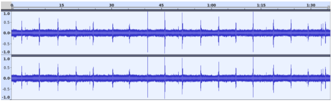
The human eye is very good at detecting patterns, and to us it’s obvious that the signal above contains repeating peaks spaced about 5 seconds apart. Those are individual bubbles going through the airlock. We can easily pick out that feature despite the continual whine of a fan plus various other background noises.

But for automated monitoring and predictability, we need to be a quantum leap more sophisticated. What’s the exact frequency of the peaks? Is the speed as expected? Is it increasing or decreasing? How would a computer fare with this data?

Unstructured data

Of course in data warehousing, there’s no such thing as entirely unstructured data. It would be impossible to read if it really was unstructured, and it would never be usable.

Rather than being completely unstructured, it’s more accurate to say that data warehouses often have to deal with data sources that are structured in complex ways. Often, that structure involves a proprietary or unusual format. Generally, it requires processing to interpret. In other words, unstructured data is hard to read!

As an example, from those 90 seconds of audio captured by the IoT device, here is a hex dump showing roughly the 1/100th of a second between 1:07.30 and 1:07.31.

f9 7d b5 20 73 d8 2f 5d d1 35 cb de 5f f4 9f ac cb 1f cd 51 41 44 f0 be c7 7e aa 29 06 d8 c4 69 e1 db 1b 3e 0b 5e ab da 4b 7a ce 80 9f 62 61 ed 42 b4 d5 51 96 d8 e9 38 c5 75 4e 51 ca 98 4e bf ed 19 7d 2e 2c 3d 9b 92 d5 64 6c 2e f5 99 29 75 ab ec b7 5a f4 39 39 30 ce 9d 91 61 4a d9 8e 57 2d 75 06 83 55 3e 3e 93 f1 c2 9d b3 48 ed f7 79 53 d9 7a 45 a8 8b 92 ef 10 57 df 95 70 44 f8 23 e5 c8 86 f5 0a 9b 94 e3 ed de 73 9c e7 44 8a 01 02 70 18 8c 8a 85 61 a1 18 1a cc 28 cd 4b 97 49 a6 5c 80 c1 48 87 8b ea 80 4d 46 1a 4a ad d5 2e 06 ba ac 42 96 b3 4d 1d 0c 61 9c 62 f5 33 62 fc 30 b1 1f af fa 68 7d 8a 58 43 a0 73 1d 07 e3 c1 b5 07 dc 3c 9f bc e9 74 e8 fe 63 bf 6f 24 9c 3b b1 db 53 24 6a 0c 2b 84 ff a2 a8 15 f5 f9 00 5b a5 0e 0f db d5 0b ff 26 1a 14 0c ad bb 9a a2 ba 52 73 37 20 d5 54 0c 31 92 9d d7 a1 91 54 6f 62 a7 35 43 a1 84 c9 99 cd 87 15 dd a1 cc f4 d6 81 d7 36 9e 07 a1 fe ed 65 7b 97 5f f7 f4 32 59 99 fe 15 31 64 ee 55 cf 15 3b f0 ff f1 4c 80 59 3f fc 21 1b 94 05 fc d4 97 ae f3 bf 8b bf 13 df eb f4 fa f8 ef a9 9a ae 72 b5 72 4b 2e 5c cb b4 a1 42 ca fc cd 6e f8 f7 f7 c6 83 c5 9c 54 7d 35 1a d3 c3 b4 9e 8e 69 da db 3b 45 b7 83 a7 ae 5d e9 88 66 4c e4 74 51 fa 5e e5 cc 73 78 bb 1a ae dc 71 7f 85 a7 6a fc 57 b0 de ef 37 f6 9b 70 73 3e

The above is only around 0.01% of the whole. The full, real data is 3MB in size–more than seven thousand times larger than this fragment.

The information must be in there somewhere, because the periodic peaks showed up clearly in the sound editor. But just looking at the bytes it is really difficult to establish that relationship. This is the first challenge for a computer dealing with “unstructured” data.

To the human eye, the bytes don’t reveal any detectable pattern. But in reality the data is organized in a logical, predictable, and fully documented way. It does have structure. In this case, you would need to know that it’s a stereo, 48KHz audio stream, exported in the AAC format. It was evidently convenient for the transducer to produce the data in that way.

There are code libraries for parsing that kind of audio data, which would be the first step in processing it. In fact, the sound editor used one of those libraries to generate the waveform image I showed at the top.

Too Much Information

In the next screenshot I have zoomed right in to highlight the same 1/100th of a second between 1:07.30 and 1:07.31. There’s no special feature at this point: it’s simply typical of the majority of the data and shows the ambient sound generated by an air fan spinning.

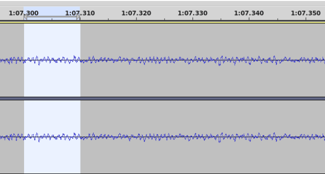
Note that, even at this large magnification, there’s still a lot of information. It could be used to check the fan speed every 100th of a second throughout the sample. This part of the signal is completely irrelevant to the problem of peak detection: It’s just some rather annoying noise. However, it would be music to the maintenance engineers, because if the fan speed changes it probably means it’s about to break and should be replaced.

Next here’s another zoom in, around the 1:33 mark this time. You can just about tell by eye that the highlighted section is not a “bubble-shaped” peak. Also it’s out of sequence, being only two seconds before the next one instead of around five seconds.

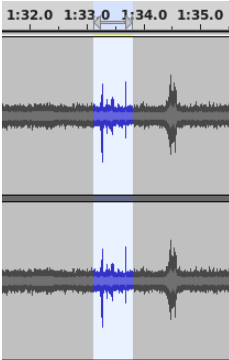
In fact, this signal has nothing to do with the chemical reaction, either. It is the audio transducer picking up the click of a door closing in the distance. Perhaps of interest to the security team? But again, irrelevant to the problem of peak detection. Distinguishing between two fairly similar-looking events is a good example of a typical difficulty that a machine learning algorithm would need to overcome.

Clearly there’s a huge amount of information contained in the data, although most of it is not useful for monitoring the chemical reaction.

Unstructured data summary

Sound is just one example of “unstructured” digital data originating from analog sources. The example I have been using is a sound recording taken from a factory floor. Human conversation is another very common source of recorded sound. Two other big categories of “unstructured” analog media are images (such as photographs, medical scans, and handwritten documents) and video (such as security or traffic monitoring).

Many “unstructured” data formats also exist that originate from digital sources. Examples include:

• PDF – the primary purpose is for display, not for data exchange
• Office productivity formats – often proprietary, undocumented or otherwise inaccessible; for example OpenOffice, Excel, or Google Sheets
• Reports and Dashboards – again the primary purpose is for display, so it’s usually difficult or impossible to acquire the original data
• Web Pages, the subject of an ongoing battle between the sophistication of scrapers and the dynamic abilities of websites
• Domain specific data, for example spatial data, with its wide range of formats including Shapefile andGeoTiff
• Exports or data dumps from databases – even if the original source was structural, the formats are usually bespoke and hard to read

Some general features are common to all “unstructured” data:

• It’s not really unstructured: Rather it is structured, but:
  • The format was chosen solely by the producer, and simply because it was the most convenient format for the producer
  • The data is non trivial to consume, often requiring special in-depth knowledge, or information that’s not present in the data
  • The data is often fairly messy
    • For analog sourced data, there is background randomness to filter out
    • For digitally sourced data, the consumer must work to separate the content from the presentation
    • Useful information density is low
      • The primary goal of the format is not the efficient exchange of information
      • The producer of the data almost certainly did not have your specific use case in mind, so useful data will usually be bundled alongside large amounts of other, irrelevant data
      • The formats are usually bulky

      A note on two categories that look unstructured:

      • Encrypted data, which deliberately does not contain enough information to read the data without the secret key
      • Compressed data, which requires that you know which algorithm to use to decompress it

      Those formats are not really “unstructured” because they almost always decrypt, or uncompress, into structured or semi-structured data.

      Semi-Structured Data

      A quick recap of the problem underpinning this article: I’m trying to monitor the rate of a chemical reaction by measuring the frequency of bubbles passing through an airlock.

      The “unstructured” audio data described in the previous section did contain all the necessary information. But it was difficult to read, and it required a layer of feature detection (a machine learning algorithm) to automatically find the peaks representing the bubbles. A better transducer, with machine learning capabilities built in, could detect those peaks itself and just output the times of the bubbles.

      In other words, what I’d prefer is the data to be presented in a more accessible way. This is the essence of semi-structured data.

      Semi-structured data is always presented in a well defined format, with agreed rules, which are convenient for both the reader and the writer. Often the data is tagged, or marked up, in a standardized way. One of the most common examples of this is JSON

      Here’s the same data again, showing just the audio peaks detected by a more sophisticated transducer, and expressed in the semi-structured JSON format.

       < "metadata": < "timestamp": "2021-10-01 23:40:02", "equipment": "M4FUI7fcnQiBs6Cg4RjztczHzrtecC7boW6oLSOa", "id": "l0oaBnUoAaAMWBEorpMs", "timeunits": "seconds", "tempunits": "celsius", "base": "2021-10-01" >, "data": [ < "timestamp": "15:18:10.532", "delta": 3.504, "temperature": 19.77899 >, < "timestamp": "15:18:15.503", "delta": 8.475, "temperature": 19.76917 >, . more of the same . < "timestamp": "15:19:41.552", "delta": 94.523, "temperature": 19.79395 >] >

      The first thing to notice about this semi-structured format is that it is both machine-readable and human-readable. It’s far easier than trying to interpret the bytes in the audio recording.

      The content of the JSON is highly selective and highly targeted. For example, there’s nothing about fan speed (let alone monitoring it every 100th of a second), or about doors opening and closing. Most of the irrelevant minutiae from the audio data have been filtered out.

      As a result of preprocessing and of being selective, the useful information density is much higher. Expressing the measurements digitally means the entire JSON document is only around 1.5Kb in size. That is nearly 2,000 times smaller than the original “unstructured” audio data.

      One thing you probably noticed is that now there are temperature readings. Where did they come from? Well it turned out that the more sophisticated transducer also had the ability to measure temperature, and it just went ahead and added those measurements to the data.

      This is a classic illustration of the fact that the writer can – and will – independently decide what information to place into semi-structured data.

      This is known as schema on read.

      Semi-structured data formats are highly flexible within the constraints of the format. If the producer adds new data, it will not invalidate anything or violate any constraint.

      Exactly the same principle applies whenever the writer unanimously decides to change the way it writes the data.

      • It might be a semantic modification such as using degrees Fahrenheit instead of Celsius.
      • Or a structural modification such as splitting the data into two arrays: one for the timings and one for the temperatures.

      This is known as schema drift.

      Alternative formats

      There’s nothing special about JSON as a semi-structured format. JSON is very widely used, but there are other common formats too.

      For example, here’s the same data expressed as YAML. It’s slightly more compact, although there’s a heavy reliance on whitespace, which can make it a little more difficult for a human to read.

      --- metadata: timestamp: '2021-10-01 23:40:02' equipment: M4FUI7fcnQiBs6Cg4RjztczHzrtecC7boW6oLSOa id: l0oaBnUoAaAMWBEorpMs timeunits: seconds tempunits: celsius base: '2021-10-01' data: - timestamp: '15:18:10.532' delta: 3.504 temperature: 19.77899 - timestamp: '15:18:15.503' delta: 8.475 temperature: 19.76917 . more of the same . - timestamp: '15:19:41.552' delta: 94.523 temperature: 19.79395 

      XML is another semi-structured format, older but still widely used. Here is the same data again. It is more highly formatted and bulky, but very easily readable. The representation of embedded lists in XML is one area that requires slightly more expensive parsing.

         2021-10-01 23:40:02 M4FUI7fcnQiBs6Cg4RjztczHzrtecC7boW6oLSOa l0oaBnUoAaAMWBEorpMs seconds celsius 2021-10-01   15:18:10.532 3.504 19.77899  15:18:15.503 8.475 19.76917  . more of the same . 15:19:41.552 94.523 19.79395   

      Semi-Structured data summary

      A wide variety of semi-structured data formats are in common use. They form a spectrum in which some are closer to “unstructured” data and some closer to “structured” data.

      More like “Unstructured”

      EDI, protobuf, HTML

      Parquet, CDW internal e.g. SUPER, VARIANT etc

      JSON, XML, YAML, Ion, XHTML

      More like “Structured”

      Some general features are common to all semi-structured data:

      • It’s highly structured, but in a flexible way which allows endless wriggle room for changes – known as “schema drift“
        • The format is easy for the consumer to handle
        • The writer may have to go to some lengths to extract the relevant information, especially if the original source was analog
        • The data is highly targeted
          • It is entirely digital
          • The content is embedded within the presentation by means of defined markup or tagging
          • Information density is high
            • The primary goal of the format is the structured exchange of information

            The actual data can only be discovered by going ahead and reading it – known as “schema on read“

            Semi-structured data solves the presentation problem by using a format that’s easy to consume. Also, semi-structured data tends to focus on specific items of data.

            Between them, those two things generally result in much higher information density than is found in equivalent “unstructured” data.

            There is a common objection that converting from “unstructured” to semi-structured data involves the loss of huge amounts of information. This is true, and is one of the costs of obtaining high information density. I can no longer monitor fan speed, for example, using the semi-structured JSON data shown in this section. That information has simply been lost.

            However a typical counter argument would be that the background fan speed did not significantly change throughout the entire day, so there’s no point repeating the same measurement over and over. It would be much simpler to replace those megabytes of analog signals with a single tiny extra piece of semistructured data – for example like this:

            "metadata": < "timestamp": "2021-10-01 23:40:02", "fan speed": "normal", "equipment": "M4FUI7fcnQiBs6Cg4RjztczHzrtecC7boW6oLSOa", 

            From the consumer’s perspective, the main difficulty with semi-structured data is that the content is always somewhat unpredictable. It’s always easy to parse, but you never know quite what information is present until you actually read it. If the writer decides to change something, they will probably just go ahead and do that with no warning.

            It always falls to the consumer to interpret the content and convert it into a format that’s fully structured. The transformation task is to look for the data you need from among the data that has actually been supplied.

            Structured Data

            This is the gold-standard format in terms of long term storage and usability. It is very compact and it is easy to retrieve and manipulate structured data, especially using SQL

            Whenever you are working with structured data, there are four strong implicit expectations:

            1. The data is tabular – i.e. rows and columns, and every single row in a given table has the exact same columns
            2. The data is relational – i.e. there may be constraints such as uniqueness (known as primary keys), and references between tables (known as foreign keys)
            3. All the column values are simple – i.e. lists and substructures are not permitted
            4. The writer and the reader agree on the structures beforehand. This is known as schema on write.
               1. The writer can’t unanimously decide to change the data model
               2. The reader can’t expect the writer to send any data that’s not in the data model

               The data structures that have been agreed upon are known as the schema or the data model. A relational data model for the purposes of this article might look like this:

               

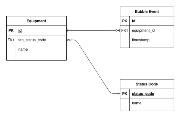
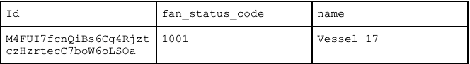
               The device generating the data is a piece of “equipment” with a serial number or primary key identifier of M4F…SOa. This is the thing that contains the fan and the airlock, plus all of the chemicals. There’s only one row, but nevertheless, the structured data for this table might look like this:

               

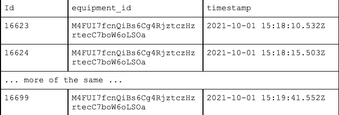
               To measure how fast the reaction is going, it’s necessary to count the frequency of the bubbles going through the airlock. In this model every single bubble has its own record in a “bubble event” table. Structured data for this table might look like this:

               

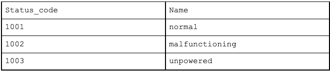
               The equipment table above had a foreign key reference 1001 to a “status code” table, which might look like this:

               

               Storing data in this way results in very high information density. Structured data exchange formats, such as CSV, look almost exactly like the above tables.

               You should recognize virtually all of the values in the above tables from the semi-structured examples in the previous section. The data is not absolutely identical, however. It does require a little transformation work to get it into that shape.

               Transforming data into structured format

               One of the first transformations is always to get the data into the correct table. A transducer counting bubbles might not be aware that it’s part of a piece of equipment labelled M4F…SOa, and certainly not that the equipment is named Vessel 17. That information must have come from somewhere else, and it has to be tracked down and sourced.

               In the JSON data I showed earlier the transducer only recorded timestamps at the detailed level. The date part was held elsewhere, and the time zone was not present at all. So to convert 15:18:10.532 into 2021-10-01 15:18:10.532Z requires data from different levels of the semi-structured output, plus some implicit knowledge that is not present in the data. Navigating granularity and locating and interpreting data are typical transformation tasks.

               Converting data into structured format also means that – at the very least – all of the normal relational rules must be followed.

               • You must create explicit primary keys if they were not present in the data. An example is the 16623, 16624 … 16699 series in the “bubble event” table above.
               • You have to decide how to handle events that appear to be duplicates. For example, if there were two events listed at exactly 15:18:10.532, should you record them both, or ignore one? Or should you ignore the whole dataset and report that the transducer is not working properly? This is an example of a business rule related to data quality.
               • You are not permitted to store values which break foreign key referential integrity. For example if you were told that the fan speed was “normal,” then the appropriate fan_status_code would be 1001. But what if you received the value “excellent” or “100%” for the fan speed? Are they the same as “normal”? Are all the “normal” fans actually malfunctioning? These are more examples of business rules.

               Structured data summary

               The most common structured format for data exchange is CSV. It is very well defined, with clear presentation rules, and is an excellent, convenient format. It’s easy to read and has a very high information density, with almost no overhead used by markup.

               A common variant is TSV, which simply means the column values are TAB-separated rather than comma-separated. The theory is that TABs are rare inside the actual data so they are safe to use as delimiters.

               Although JSON is really a semi-structured format, there is one variation in which multiple documents (i.e. “rows”) are held in a single file, with the expectation that the same fields (i.e. “columns”) occur in all the documents. This is known as “JSON Lines”, JSONL, LJSON or sometimes NDJSON. It has the advantage of solving the main structural schema drift problem that CSV can be vulnerable to – when the column ordering is inadvertently changed.

               The general features listed below are common to all structured formats:

               • It’s highly structured, tabular, and in a format prearranged between producer and consumer – the data model
                 • Structured formats are easiest for the consumer to read, although they are usually more difficult for the producer to create
                 • Consumers are still vulnerable to unannounced semantic schema drift. For example, the producer could silently switch from using degrees Celsius to degrees Fahrenheit, without changing the structure at all
                 • If you are encountering structural schema drift, it’s likely that you are actually dealing with a semi-structured data source masquerading as a structured data source
                 • The data is highly targeted
                   • It is entirely digital
                   • Minimal presentation is used: The content is almost exclusively made up of the data itself
                   • Information density is very high
                     • The primary goal of the format is the exchange of information in predefined structures
                     • You don’t have to read the data to determine the actual contents–this is known as “schema on write“

                     Schema drift does (and should!) still happen sometimes, even with structured data. It’s a good indication that change and growth are happening in the source systems. The ideal is when the schema drift is governed, and both the producer and the consumer are part of the change management process.

                     Summary

                     Having looked at the same data represented in all three different ways, it’s clear that unstructured data is most convenient for the producer (the writer) of the data, whereas structured data is most convenient for the consumer (the reader). Semi-structured data is always presented according to agreed rules, but the actual content can only be discovered by reading it.

                     Presentation optimal for	Content optimal for
                     Unstructured	Writer	Writer
                     Semi-structured	Reader	Writer
                     Structured	Reader	Reader

                     Information density and useability both increase as data moves towards structured formats. The next chart shows what kinds of transformations need to be done to convert unstructured and semi-structured data into structured data.

                     

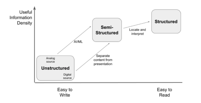
                     Applying these transformations makes the data adhere more strongly to a schema or a data model. When data becomes structured, it becomes highly consumable and highly consistent. Structured data with a well defined data model is a dependable platform upon which to build reliable insights.

                     Try it for yourself

                     You can download the sample data files used in this article.

                     • semi-structured-example.json – Semi-Structured example as JSON
                     • semi-structured-example.xml – Semi-Structured example as XML
                     • semi-structured-example.yaml – Semi-Structured example as YAML
                     • unstructured-example.aac – The original “unstructured” audio file

                     Matillion ETL can help you ingest, transform, and integrate a wide variety of structured, unstructured and semi-structured data. To see how Matillion ETL could work with your existing data ecosystem, request a demo.